Klotzbach Revisited

Guest blog by Jos Hagelaars. Dutch version here.

The average surface temperature of the earth, measured by ‘thermometers’, are released by a number of institutes, the most well-known of these datasets are GISTEMP, HadCRUT and NCDC. Since 1979 temperature data for the lower troposphere are released by the University of Alabama in Huntsville (UAH) and Remote Sensing Systems (RSS), which are measured by satellites.
The temperatures of these two methods of measurement show differences, for instance: the NCDC data indicate a trend over land of 0.27 °C/decade for the period 1979 up to and including 2012, while over the same period, the trend based upon the satellite data by UAH over land is significantly lower at 0.18 °C/decade. In contrast, the trends for global temperatures indicate much smaller differences, for NCDC and UAH these are respectively 0.15 °C/decade and 0.14 °C/decade for the same period.

Big deal? Almost everything related to climate is a ‘big deal’, so it is of no surprise that the same applies to these trend differences. In a warming world it is expected that the temperatures of the upper troposphere increase at a higher rate than at the surface, regardless of the cause of the warming. The satellite data (UAH and RSS) do not reflect this. Why is the upper troposphere expected to warm at a higher rate and what is the cause of these trend differences between the surface  and satellite temperatures?

The temperature gradient in the troposphere / the ‘lapse rate’

When you go up in the troposphere it gets colder. This is caused by the fact that rising air will cool down with increasing altitude due to a decrease in pressure with altitude, by means of so-called adiabatic processes. This temperature gradient is called the lapse rate, a concept one will frequently encounter in papers regarding the atmosphere in relation to climate. When the air is dry, this temperature drop is about 10 °C per km. When the air contains water vapor, this vapor will condense to water upon cooling as a result of the rising of the air, which releases heat of condensation. So in this way, heat is transported to higher altitudes and the temperature drop with height will decrease. For air saturated with water vapor, this vertical temperature drop is approximately 6 °C per km.

When the earth gets warmer, air can contain more water vapor. This also has an impact on the lapse rate, since more water vapor means more heat transfer to higher altitudes. This effect on the lapse rate is called the lapse rate feedback. More heat at higher altitudes implies that there will be more emission of infrared light, a negative feedback. This effect is particularly important in the tropics. At higher latitudes, the increase in temperature at the surface is dominant, therefore the change in the lapse rate will turn into a positive feedback. See figure 1 (adapted from the climate dynamics webpage of the University of Leuven).

Figure 1. A schematic representation of positive and negative lapse-rate feedbacks.

On average it is expected that the negative lapse rate feedback will dominate, leading to an overall value of about -0.8 W/(m²·K) (Soden and Held 2006 or IPCC 2007).

The satellite temperatures are by no means a representation of surface temperatures; they represent some sort of average of the entire lower troposphere. The temperature values are derived from the microwave radiation of oxygen from different heights in the atmosphere. See figure 2 for the weighting functions against altitude of the RSS temperatures for the lower troposphere (TLT). These weighting functions are different for land and ocean areas.

Figure 2: The weighting functions against altitude for the RSS TLT data.

Since it is expected that the average lapse rate feedback will be negative, the temperature aloft should on average increase more than at the surface (because when it gets warmer, more heat will be transported to higher altitudes). As mentioned above, this is however not corroborated by the comparison between surface and satellite temperatures.

These differences have been a regular subject of research. The most well-known investigations are Santer et al 2005, Karl et al 2006 and a review by Thorne et al 2011.

Santer et al concluded that on monthly and annual time scales the temperature observations of the troposphere in the tropics were consistent with the theory and show a greater warming at a greater height than at the surface. However on a time scale of decades, they only encountered one dataset that met these expectations, as can be seen in figure 3 (adapted from Thorne 2011).

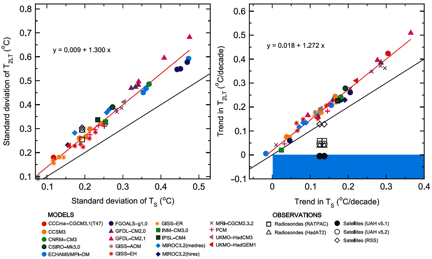
Figure 3: Tropical temperature behavior in observations and models.
The black line in the graphs indicates an amplification factor of 1 for the surface temperature (Ts) to the temperature of the complete lower troposphere (2LT);the red line denotes an amplification factor of about 1.3 (slope of model expected tropospheric versus surface temperatures).
The graph on the left is a representation of the month-to-month variability, were the models and the observations (radiosonde data, satellites and surface temperatures) are in agreement.
The graph on the right is a representation of the trends on a multi-decadal scale. Here the models also show an amplification factor of about 1.3, whereas the observations show a smaller amplification factor, in some cases even smaller than 1.

The extensive report of the U.S. Climate Change Science Program (Karl et al) concluded:
These results could arise due to errors common to all models; to significant non-climatic influences remaining within some or all of the observational data sets, leading to biased long-term trend estimates; or a combination of these factors. The new evidence in this Report (model-to-model consistency of amplification results, the large uncertainties in observed tropospheric temperature trends, and independent physical evidence supporting substantial tropospheric warming) favors the second explanation.

So, a deviation in the long-term trend in the observations would be the most likely explanation for the trend differences. Looking specifically at the satellites, this is not illogical given the difficulties inherent to satellite measurements (see e.g. the various UAH versions), such as the drift in the satellites’ orbit, sensors which deteriorate over time, calibration problems when changing from one satellite to another, or temperature effects in the instruments themselves. Even last year Po-Chedley & Fu found another bias in these satellite temperatures, and one of their conclusions was:
“Creating climate-quality satellite temperature datasets is a challenging process that requires constant attention as new biases are discovered.”

Klotzbach 2009

In 2009 a paper was published in the Journal of Geophysical Research by Klotzbach, Pielke Jr. and Sr., Christy and McNider, with the title:
“An alternative explanation for differential temperature trends at the surface and in the lower troposphere”.
Their general conclusion was:
“The differences between trends observed in the surface and lower-tropospheric satellite data sets are statistically significant in most comparisons, with much greater differences over land areas than over ocean areas. These findings strongly suggest that there remain important inconsistencies between surface and satellite records.”
The Klotzbach-2009 paper implies that these ‘inconsistencies’ are caused by biases in the surface temperatures, see their paragraph 2 with the title: “Recent Evidence of Biases in the Surface Temperature Record”.

To assess the trend differences between NCDC/HadCRUT3 and the UAH/RSS data, they took the monthly values of the different datasets, subtracted these from each other and calculated a trend over these monthly differences. This trend should be 0 when there is no difference between the datasets. Figure 4 contains the results from the Klotzbach-2009 paper (their table 2).

Figure 4: Differences in trends between NCDC/HadCRUT3 and UAH/RSS over 1979-2008.

The biggest difference was obtained for NCDC minus UAH with a trend of +0.15 °C/decade over land and +0.04 °C/decade for the globe as a whole, for which a negative ratio would be expected. This is consistent with the conclusions drawn by Santer et al that the multi-decadal trend is anomalous, whereas the same anomaly is not apparent on shorter time scales. This led them to state the following: “The real conundrum is the complex behavior of the observations”.

The same calculations were performed in Klotzbach-2009 with an amplification factor for the warming at higher altitudes, which obviously lead to even greater differences. They used an average amplification factor of 1.2 which the authors had obtained from Ross McKitrick, via data from a GISS-ER climate model study (copied from an FTP server). This trick caused some turmoil, see e.g. this RealClimate blog post. Gavin Schmidt (responsible for the GISS climate model) came to entirely different conclusions based on his model, namely an amplification factor of 0.95 on average over land and 1.4 over oceans (instead of the 1.2 for the globe as a whole used by Klotzbach-2009). In 2010 a correction was published with respect to the original paper, in which the calculations were repeated with an amplification factor of 1.1 above land and 1.4 above the oceans. Oddly, the value of 0.95 as calculated by Schmidt (see this e-mail exchange) was not used.

Sometimes Klotzbach-2009 is used in climate skeptic texts to indicate that there are problems with the measurements of surface temperatures and that these measurements cannot be trusted. For instance, the skeptical Dutch journalist Marcel Crok used the trend of 0.15 °C/decade from figure 4 in his book “De staat van het klimaat”. For Dutch readers, see this review of this part of Crok’s book on ‘PCCC klimaatportaal’, which contains the following quote [my translation]:
“If there were a ‘bias’ in the surface measurements, then satellite and surface measurements should deviate more and more in the course of time, shouldn’t they? […] and indeed this appears to be the case. Over land, the difference between the temperature measurements and the satellite measurements has risen to 0.5 degrees over the past thirty years. Whilst climate researchers expect the opposite.”
His 0.5 degrees is presumably based on three decades times 0.15, rounded up to 0.5 °C; note that only the highest number in the table of Klotzbach-2009 (the above Fig. 4) has been used. The two types of measurements over land deviate, and according to Gavin Schmidt, surface temperatures over land are expected to be slightly larger than tropospheric temperatures. Moreover, Crok omits the possibility that there could also be a ‘bias’ in the satellite measurements.

Anthony Watts also references to Klotzbach-2009, he writes in his 2012 paper based on his Surface Stations Project:
By way of comparison, the University of Alabama Huntsville (UAH) Lower Troposphere CONUS trend over this period is 0.25°C/decade and Remote Sensing Systems (RSS) has 0.23°C/decade, the average being 0.24°C/decade. This provides an upper bound for the surface temperature since the upper air is supposed to have larger trends than the surface (e.g. see Klotzbach et al (2011). Therefore, the surface temperatures should display some fraction of that 0.24°C/decade trend. Depending on the amplification factor used, which for some models ranges from 1.1 to 1.4, the surface trend would calculate to be in the range of 0.17 to 0.22, which is close to the 0.155°C/decade trend seen in the compliant Class 1&2 stations.
Here an amplification factor of 1.1 to 1.4 (from the Klotzbach-2010 correction paper) is used, while for over land this should be a bit lower than 1. After all, the USA should be categorized under ‘land’ and not under ‘ocean’. Phrases like these, not supported by valid research, should, in my humble opinion, not be published.

4 years later in 2013

2012 has passed and now we have 4 more years of data than back in 2009. Not much has changed regarding the surface temperatures, except some small improvements in the homogenization and the integration of more measurement stations (e.g. HadCRUT4 instead of HadCRUT3). These changes have not resulted in significantly different trends for the global temperatures. The transition from GHCN-M (Global Historical Climatology Network-Monthly as used for e.g. the NCDC temperatures) from version 3.1 to version 3.2 has even led to a higher trend for the land temperatures (having changed from 0.94 °C/century to 1.11°C/century for NCDC for example), with the largest differences before 1970. In addition, the surface temperatures over land of the three aforementioned institutes,  are consistent with the temperature results from the BEST project led by Richard Muller.

So, the trends in surface temperatures have not changed dramatically, though may have slightly increased in some cases. If the climate skeptic fans of the Klotzbach-2009 article are correct regarding there being strong biases in the surface temperatures, these temperature differences should therefore have increased even further.

Anyone with a spreadsheet program and an internet connection is able to redo the calculations of Klotzbach-2009 and verify whether the expected temperature difference has increased. This also applies to me and my results are shown in figure 5. The uncertainty is calculated according to the method as described in Foster & Rahmstorf 2011.

Figure 5: Differences in trends between NCDC/HadCRUT4 and UAH/RSS over 1979-2012.

We now have 13% more data and the trend difference over land between NCDC and UAH has decreased with approximately 33% from 0.15 to 0.10 °C/decade. This would translate in a divergence between surface and tropospheric trends of 0.34 °C over 34 years; less than Crok’s estimate of a few years ago.
Still, over land the trend in surface temperatures is significantly larger than in satellite temperatures. Over the oceans, the GISS model results indicate that the surface should warm significantly more than the troposphere (by a factor of 1.4); this is not seen in the observations, so also for those areas an interesting puzzle remains.
The HadCRUT4 data indicate greater differences than the old HadCRUT3 data and are, as expected, much more in line with the NCDC data.
The math in the book of Marcel Crok now generates a difference in surface minus tropospheric trends of 0.24-0.34 °C over 34 years. The average difference is 0.3 °C and is significantly lower than the 0.5 °C he mentioned in his book.

Conclusion

The expected increase in the differences between the surface temperatures and the satellite temperatures over land has not occurred. To the contrary, 13% more data show that the trend difference over land has decreased by 18% for NCDC/RSS and by 33% for NCDC/UAH.
The trend difference has thus decreased rather than increased, and whereas Klotzbach-2009 and its fans champion the argument that this difference is due to a ‘bias’ in the surface temperature record (some 1700 words were spent on this argument in K-2009), a ‘bias’ in the satellite record may be equally, or perhaps even more plausible.

Be warned if in blog pieces or papers the amplification factors between the temperatures at the surface and higher up in the troposphere are (improperly) used.

Many thanks to Bart for helping me out with the translation and for constructive comments. A reply to this blog post (or rather, to a google translation of the original Dutch post) by Klotzbach’s co-author John Christy has been posted by Marcel Crok and reposted at WUWT. A reply to John Christy is forthcoming.

For more information, see:

– The Idso’s on CO2Science
– Blog Roger Pielke Jr.: here, here and here
– ClimateAudit
– SkepticalScience: here and here
– RealClimate: here and here
– Press release Po-Chedly en Fu
– MET Office HadAT2 vs MSU
– Critiques and discussions: here, here, here and here
– The IPCC about water vapor and lapse rate

Tags: Christy, Klotzbach, McNider, Pielke, satellites, surface, temperature trend, troposphere